The machine got wider, not faster
Why linear programming had to change algorithms to use a GPU.
A linear program is a planning problem in which everything is proportional: a workshop with limited stock, several things it can build, a known profit for each, and the question of how much of each to build. Since the 1940s the standard way to solve one has been the simplex method, which walks from corner to corner of the region of legal plans, improving as it goes, and stops when no neighbouring corner is better. The previous guide builds it; all you need here is that shape: a walk, one step at a time.
Two methods. Same small workshop, same starting point, same step sizes. Their inner loops cost exactly the same to run, and the code differs by one term in one line.
One of them lands on $350, which is the right answer.
The other never lands on anything at all. Four thousand iterations in, it is still swinging between $0 and $753, and it would still be swinging after four million.
One term. That is the entire difference between a method and a thing that spins forever.
Nobody puts up with something that delicate unless they are being forced to, so the first question is what is doing the forcing. It is the hardware. For thirty years the way to solve a linear program faster was to buy a quicker processor. That stopped working. What replaced it was not a quicker processor but a much wider one: thousands of arithmetic units, fed by a memory system that did not get thousands of times faster.
And the simplex method cannot use a machine like that. Not for want of anyone trying — it is a chain of decisions where each one depends on the last, and a machine that can do ten thousand things at once is no help whatever when you have exactly one thing to do until it finishes.
So the interesting question is not how to parallelise simplex. It is what a method would have to look like to use that hardware at all, and what you give up by using it. The delicate one is the answer, and the missing term is where the guide is going.
The plan. Chapters 1 and 2 are about the hardware and why it changes which algorithms are worth having. Chapter 3 is why simplex is the wrong shape. Chapters 4 to 10 build a method that is the right shape, starting from the version that does not work. Chapters 11 and 12 are whether it gets the right answer and what it costs.
Every number below is computed by the code in this folder. The answers it is checked against come from the exact rational simplex in the duality guide, which shares no line of code with anything here.
0What this is
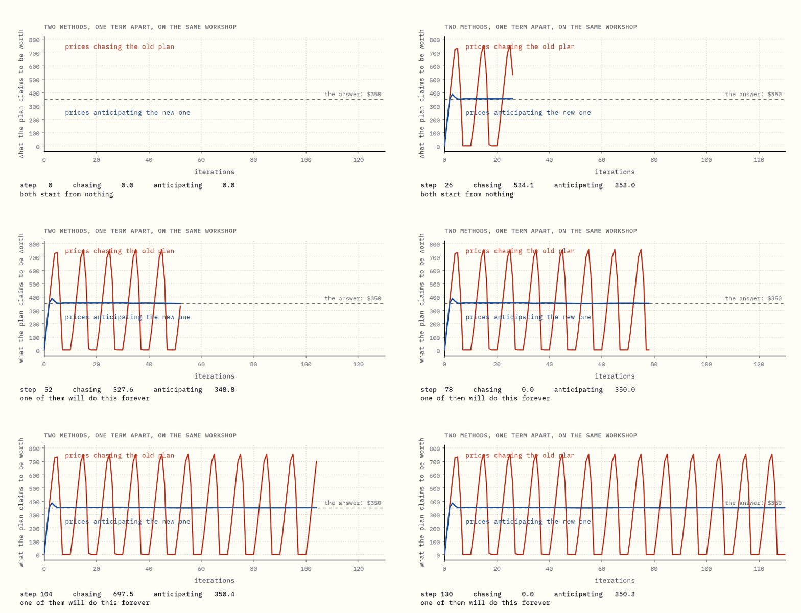
Each curve is what one method believes its current plan is worth, plotted against how many rounds of arithmetic it has done. The problem behind them is a workshop with three shelves of raw material and two things it can build, small enough that the right answer is known exactly and is $350.
The blue one climbs and stops on $350.
The red one never settles. Four thousand rounds in it is still swinging between $0 and $753, and it will keep swinging forever.
Now the part that makes this worth a guide. Neither curve is a bug, and neither method is badly tuned. They were given the same problem, the same starting point and the same step sizes, and their two update rules are identical except for a single extra term in one line. That one term is the difference between a method that works and a method that does not exist.
Both of these methods are built the way they are for one reason: their inner loop is nothing but multiplying a table of numbers by a list of numbers, over and over. That is the one kind of work a graphics processor can do thousands of ways at once, and it is why anybody tolerates a method this fragile. The guide is the case for that trade: what the hardware demands, what a method shaped to satisfy it looks like, what the missing term is, and what you give up by taking the deal.
In one sentence. There is a method that can use parallel hardware, but only just, and what separates it from a method that never converges is one term in one line.
1How much arithmetic per byte
Start with the hardware, because it decides which algorithms are worth having, and it decides it before you have written a line.
A modern accelerator has enormously more arithmetic capability than a server processor. It does not have proportionally more memory bandwidth. Roughly: a hundred times the arithmetic, but only about fifteen times the rate at which it can fetch numbers to do arithmetic on.
So a machine has two speeds, and which one you get is a property of your work rather than of the machine. A single question decides it.
How much arithmetic do you get to do for every byte you had to fetch to do it?
Multiply two dense matrices and the answer is enormous: every number you load is used hundreds of times over, so the arithmetic is the thing you are waiting for. Add two long lists of numbers and the answer is dismal: load sixteen bytes, do one addition at 0.06 operations per byte, move on, and the arithmetic units spend almost all of their time waiting for the next delivery. Everyone calls this ratio arithmetic intensity.
Now count it for the operation this whole guide is about.
Multiplying a sparse matrix by a vector, the way solvers store matrices, costs about 12 bytes per stored entry: eight for the value and four to record which column it sits in. Having fetched that entry, you do 2 operations with it, one multiply and one add. Then you never look at it again. There is no reuse anywhere in the operation, which is exactly what "sparse" costs you.
Two operations per twelve bytes. 0.17 operations per byte.
A vector add is poorer still, at 0.06, but nobody builds a solver out of vector adds. For the operation an LP solver actually spends its life in, 0.17 is as low as it gets, and everything in the next chapter follows from it.
In one sentence. A sparse matrix-vector product does one sixth of an operation per byte it fetches, and nothing about how it is written can change that.
2The roofline
Put 0.17 against the machines and the picture resolves.
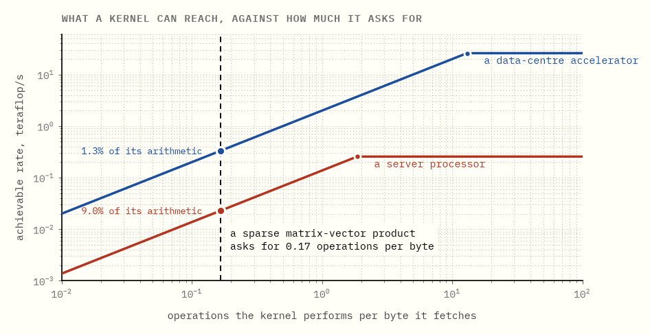
A machine has an intensity of its own, and it is the break-even point: divide its arithmetic rate by its bandwidth and you get the number of operations it can perform in the time it takes to deliver one byte. Feed it work above that number and its memory system keeps up and the arithmetic runs flat out. Feed it work below, and the arithmetic waits.
That is what the chart draws. Each machine's ceiling rises with intensity until it hits the flat roof of its own arithmetic, and the two regimes meet at that break-even point.
The accelerator can perform 13 operations for every byte it delivers. Give it work that asks for 0.17 and almost all of that arithmetic sits idle: it reaches 1.3% of what it could do, because 0.17 divided by 13 is about a hundredth. The server processor, which can perform 1.9 operations per byte, reaches 9% of its own, by the same division. Our work sits far to the left of both roofs.
Now the consequence. The accelerator is still the faster machine here, by 14.5×, and 14.5 is precisely the ratio of their bandwidths, not the ratio of their arithmetic, which is about a hundred. Both machines are being starved. The one with the fatter pipe is starved less, and by exactly the ratio of the pipes.
So for this kind of work, buying a machine with more arithmetic buys you nothing. Buying one with more bandwidth buys you what it says on the label, no more and no less.
Which tells you what a good algorithm looks like on hardware like this: one whose entire inner loop is streaming over the matrix, and which does no other kind of work at all.
In one sentence. Sparse matrix work is limited by memory bandwidth, not arithmetic, so the only speedup a wider machine can offer is its bandwidth ratio.
3Why simplex is the wrong shape
Draw every plan the workshop could legally carry out and they fill a region with flat sides and sharp corners. The simplex method walks from corner to corner of that region, and each step is a chain:
- Work out which product would improve the plan if you started making it.
- Work out how much of it you can make before some rule binds.
- Update the plan, and update the bookkeeping that made step 1 answerable.
You cannot start step 1 of the next iteration until step 3 of this one has finished, because step 3 is what changes the answer to step 1. The dependency is not incidental to the implementation; it is the method. Each corner is chosen using the information produced at the previous corner.
There is a second problem underneath. The bookkeeping in step 3 is a factorisation of the current basis, maintained incrementally, and solving with it is a triangular solve: a sequence of substitutions where each one needs the previous result. Sparse triangular solves have very little parallelism in them by construction.
None of this makes simplex a bad method. It is an extremely good method, and on most problems it is still the one to use. It is simply the wrong shape for a machine whose advantage is doing ten thousand independent things at once.
(Why interior point methods are a different shape again, and where each one wins, is the guide before this one.)
In one sentence. Simplex is a chain of dependent decisions, so its speed comes from taking few steps rather than from taking them in parallel.
4Reading the table two ways
So ask for the exact opposite of chapter 3. What would a method look like if the only thing it ever did was multiply by the matrix?
Answering that needs some notation, and this chapter spends all of it. Four
symbols, A, x, b and y, and one mark on top of the first. Nothing else
in this guide is written in symbols at all, so if you get through this chapter
the rest is English.
The problem is the workshop from the duality guide, which builds tables and chairs out of three things it has a limited amount of:
| planks | hours of work | saw time | sells for | |
|---|---|---|---|---|
| a table | 4 | 2 | 3 | $30 |
| a chair | 2 | 3 | 1 | $20 |
| in stock | 44 | 30 | 32 |
Call the six recipe numbers A: three rows, one per shelf, and two columns,
one per product. A plan is two numbers, how many tables and how many chairs,
and it is called x. The stock levels, 44, 30 and 32, are a list called b.
Read the table across, and you get Ax. A row of A is a shelf, and it
tells you which products drain it. So Ax means "run the plan through the
recipes and report what it consumes". Build 5 tables and 2 chairs and the plank
row gives 4×5 + 2×2 = 24 planks; the other two rows give the hours and the saw
time. Ax is a shopping list, one entry per shelf, and it is the thing that
has to stay under b.
So the workshop's question, written for a machine, is:
choose a plan
x, at least zero in every entry, so thatAxstays under the shelf limitsb, making the profit as large as possible.
Read the table down, and you get Aᵀy. The duality guide's second idea
gives the other half: put a price on each shelf, so much per plank, so much per
hour of work, so much per hour of saw time, and collect the three prices in a
list called y. Now a column of A is a product, and it tells you what that
product is made of: a table is 4 planks, 2 hours and 3 of saw time. Multiply a
column by the prices and add up, and you have what one table's ingredients
cost. Doing that for every column at once is what A transposed times y
means, written Aᵀy.
Transposing is not an operation performed on anything. It is a decision to read the same six numbers down instead of across. That is the whole content of the little mark, and it is the reason the method in this guide costs what it does: the two directions share one copy of the matrix, so streaming over it serves both.
A turns a plan into a bill for shelves. Aᵀ turns shelf prices into a price
per product.
One worked case you can check on the back of an envelope, using the prices that turn out to be right in chapter 11, namely $6.25 a plank, $2.50 an hour and nothing for the saw. A table's ingredients cost
4×6.25 + 2×2.50 + 3×0 = 25 + 5 + 0 = $30
which is exactly what a table sells for. At those prices, building a table breaks even to the penny. That is no coincidence, and the duality guide is where it comes from.
In one sentence. One table of six numbers, read across, turns a plan into a bill; read down, it turns prices into a cost per product.
5Two players, one score
Two readings, two half-answers. To get a method they have to be pushed against each other, and that needs a single number they can disagree about.
Score any pair of plan and prices like this:
what the plan costs, plus the prices times how much the plan overruns each shelf.
The first half is the plan's own score, with profit counted as a negative cost, so that a workshop trying to earn the most becomes a plan trying to cost the least. The second half is a fine. Overrun the plank shelf by three planks with planks priced at $6.25 and you are charged $18.75 for it. Leave planks spare and the term goes the other way, which is the prices admitting they would rather be zero on a shelf nobody is fighting over.
Now watch the two sides want opposite things from that one number.
The plan wants it small. It will happily overrun a shelf if the profit exceeds the fine, so it leans on whichever shelf is currently cheap.
The prices want it large. If a shelf is overrun, raising its price punishes the plan for exactly that, so prices climb on whatever is being abused.
Neither side is trying to find the answer. Each is only trying to beat the other. And the place they come to rest, where neither the plan nor the prices can improve by moving any further, is the answer to both problems at once: the plan is the best one, and the prices are the shadow prices of the duality guide.
That is the trick to carry out of this chapter. The optimum has been turned from something to search for into a standstill between two greedy parties.
In one sentence. One score that the plan pushes down and the prices push up turns "find the best plan" into "find where two opponents stop moving".
6A method made of one operation
Now the payoff, and it is why the last two chapters were worth the trouble. Both questions the method needs to ask turn out to be the same table, read the two ways chapter 4 set up.
To improve the plan you need to know, at the current prices, whether a product
earns more than its ingredients cost. That comparison is the profit against
Aᵀy.
To improve the prices you need to know which shelves are overdrawn. That is
Ax against b.
Two questions, two readings of the same table, one matrix-vector product each. Then you clamp anything that went negative back to zero, because there are no negative chairs and no negative prices.
That is the entire vocabulary of the method. Two matrix-vector products, some vector addition, and a clamp. No factorisation, no basis, no pivoting, no ordering, nothing sequential.
Look back at what chapter 3 said simplex could not avoid, a chain of dependent decisions and a triangular solve, and then at what chapter 2 said the hardware wants: an inner loop that does nothing but stream over the matrix. This is that loop and nothing else.
The only question left is whether it works.
In one sentence. Letting the plan and the prices take turns gives a method whose whole inner loop is two passes over the matrix.
7The obvious version does not work
The obvious thing is to move both at once. Push the plan down a little, push the prices up a little, repeat. It is the first thing anyone would write, and it does not work at all.
To see what happens, shrink the problem until the whole state fits on a page:
one variable, one rule, x = 3. Nothing to maximise, one shelf, one product,
and the plan simply has to hit 3. Then the state is a plan and a price, two
numbers, and the path they trace is a curve in a plane.
With one of each, both matrix-vector products of chapter 6 collapse to a single multiplication, and the whole method is two lines. Take the step size to be 0.2 on both sides. Each iteration does:
new plan   =  plan  + 0.2 × price
new price  =  price − 0.2 × (plan − 3)
The plan is pushed in whichever direction the price is pointing. The price
rises whenever the plan is short of 3 and falls whenever it is over. The catch
is in the second line: the plan it reads is the old one, from before the
first line ran.
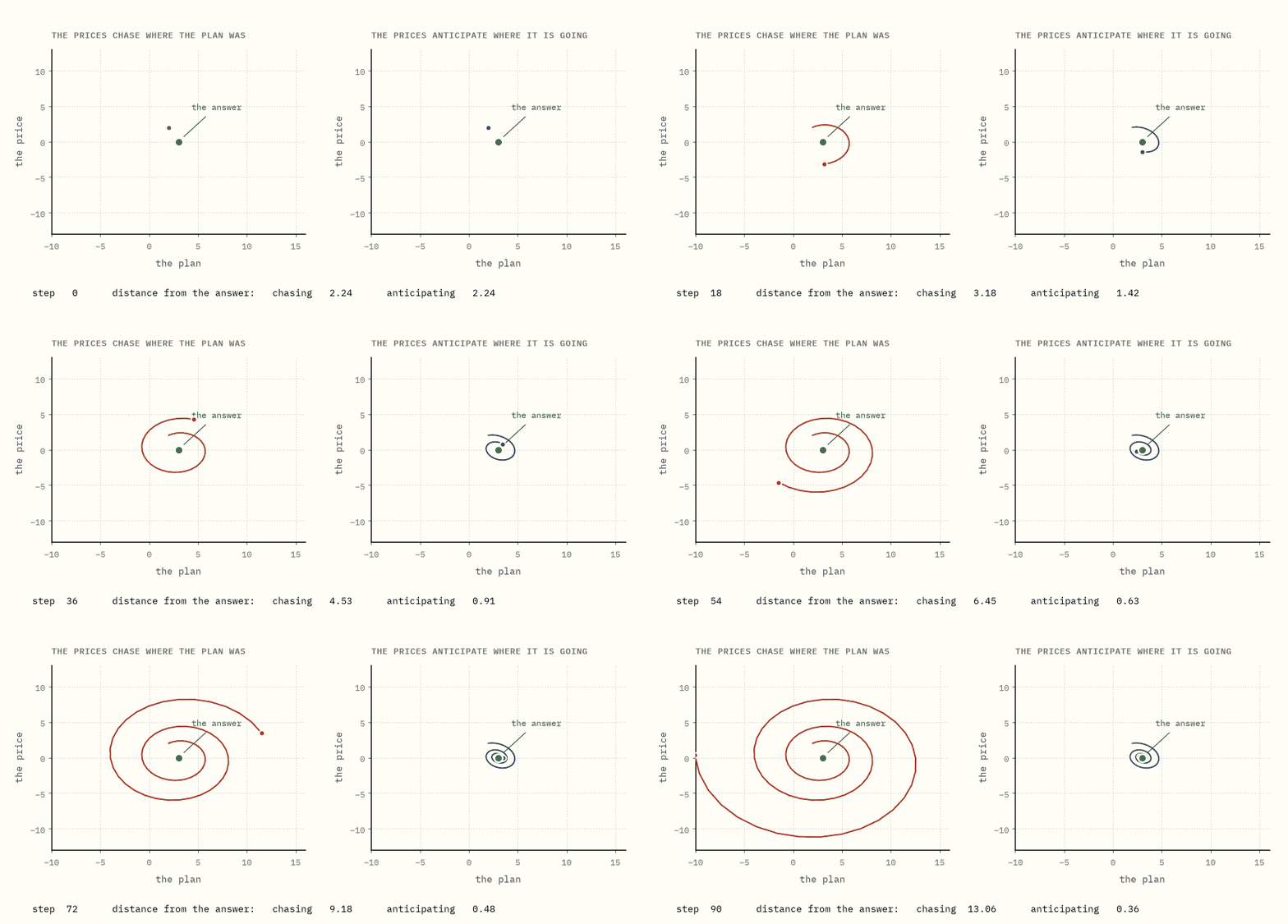
Follow it from a plan of 2 and a price of 2. The price is 2, so the plan moves up to 2.4. The plan was 2, a unit short, so the price climbs to 2.2. Next round the plan reaches 2.84 and the price 2.32. The plan crosses 3 on the third step and the price is still rising, because the plan it is being shown is the one from before the crossing. By the time the price notices and turns around, the plan is at 3.77 and sailing away.
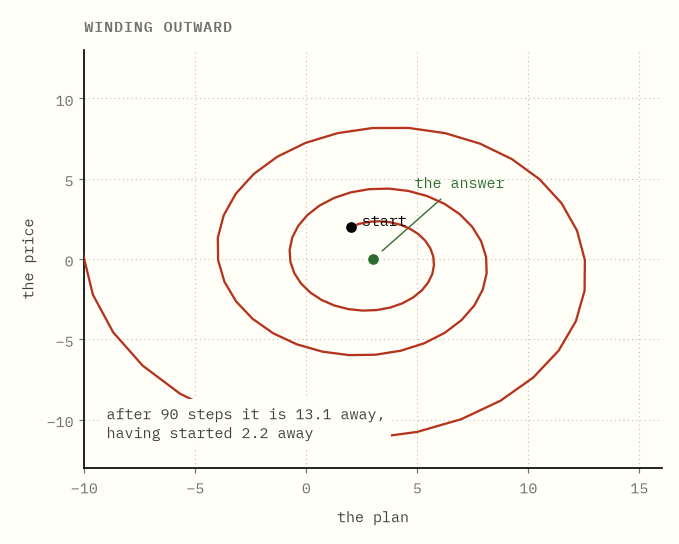
It winds outward. It starts 2.2 away from the answer and after 90 steps it is 13.1 away, and it keeps going.
Every lap is that same overshoot, in both directions, and each one is wider than the last. The two sides are not fighting each other. They are each answering a question about where the other one was, one step too late, and a pair of players who are each a step behind the other will circle forever. Nothing in the update ever notices.
On the real workshop the failure looks different and is no better. There the clamp at zero keeps the numbers from running away, and instead the method settles into an exact repeating cycle of period 10: the plan climbs to about 17 tables, the prices spike, the plan is slammed to nothing, the prices decay, and it begins again. The value it reports swings between $0 and $753, and it never once sits at $350.
So it neither runs away nor settles down, and it will carry on like that for as long as you care to let it run.
In one sentence. Two players each reacting to the other's previous move circle forever instead of settling.
8One term different
Now the fix. Brace yourself, because it is almost nothing.
When the prices react, do not show them the plan's current position. Show them where the plan is heading: the new plan, plus the step it has just taken, again.
If the plan moved from x to x′, the prices are shown 2x′ − x, which is
x′ plus the change x′ − x a second time. That is the cheapest imaginable
guess at where the plan will be next: assume it keeps going the way it was
going. On the toy problem the second line becomes
new price = price − 0.2 × (2 × new plan − plan − 3)
and nothing else changes. First step from a plan of 2 and a price of 2: the plan still moves to 2.4, but the price is now shown 2×2.4 − 2 = 2.8 instead of 2. Still short of 3, so the price still rises, but to 2.04 rather than 2.2. The correction is smaller because it arrives less late, and that is the entire repair.
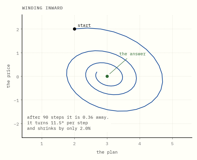
Same problem, same step sizes, same starting point, one changed term. The spiral reverses. After 90 steps it is 0.36 away instead of 13.1.
Side by side, from the same start:
This is the primal-dual hybrid gradient method, and it is the algorithm underneath the first-order LP solvers that run on GPUs.
Its per-iteration cost is unchanged: still two matrix-vector products, still no factorisation. It has not become a more expensive method. It has become a convergent one.
Try it yourself → Switch the anticipation off and watch the same code start cycling, then turn it back on and raise the step size until even that stops working.
In one sentence. Letting the prices anticipate the plan's next move rather than react to its last one turns the spiral inward, at no extra cost.
9It turns fast and shrinks slowly
The spiral converges. So we are done — except look at how it converges, because that is where the trouble is.
Look at what one step of the inward spiral does. It carries the point some way around the answer, and it brings it a little way in. A turn and a shrink, over and over.
That is not merely what the drawing looks like; on the toy problem it is precisely what the arithmetic does. There is nothing being clamped and no case analysis, so if you measure the state as an offset from the answer, one iteration is exactly multiply that offset by a fixed two-by-two table of numbers, and it is the same table, every step, forever.
A step of that kind is summarised by two quantities: how far round it carries the point, and how much it closes in. Both can be computed in advance rather than measured off a picture. With a step size of 0.2:
- it turns 11.5° per iteration, so a full revolution takes 31.2 steps (360 divided by the unrounded 11.537, not by the 11.5 printed here)
- it shrinks the distance to the answer by 2.0% per iteration
(Both come from the eigenvalues of that two-by-two matrix, which turn out to be a complex conjugate pair: the angle of the pair is the turn, and its magnitude, √(1 − 0.2 × 0.2) = 0.9798, is the shrink. Read the 2.0% as the rate the spiral settles into rather than a promise about the change in distance at each individual step. Nothing below needs the machinery, only the two numbers.)
Put them together and the difficulty is plain. Thirty-one steps of shaving 2% off a distance leave you about half as far away as you began, so one full revolution of that spiral buys you one halving. It is spinning quickly and closing in barely at all.
The obvious reply is to take a bigger step, and on this toy the obvious reply is right.
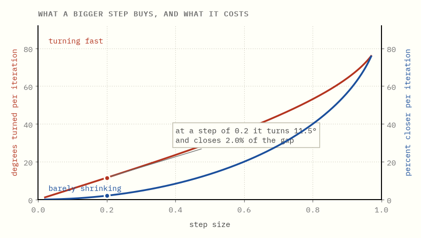
Both curves rise together. At a step of 0.9 the same iteration shrinks the distance by 56% per step instead of 2%, and it is still perfectly stable. Ninety steps then leave you at 10⁻³³ rather than 0.36. So on one variable and one rule there is no bind at all: turn the step up until just before it breaks, and go home.
The bind arrives when A stops being a single number.
Here is the thing a matrix has that a number does not. Stretch the plane by A
and some directions get stretched more than others; the largest of those
factors and the smallest are what the method has to live between. For the
workshop they are 6.33 and 1.71.
Now watch those two numbers fight over one step size.
The largest sets the speed limit. The iteration is only stable while the step stays under one over the biggest stretch. Exceed it and the spiral turns outward again, exactly as in chapter 7. So the step is capped at roughly 1/6.33, and every direction has to use that same cap.
The smallest sets the pace. How fast a direction converges depends on its own stretch factor, not on the biggest one. At the largest safe step, the 6.33 direction contracts a comfortable 56% per iteration. The 1.71 direction contracts 3.0%.
The slow one is the one you wait for. It does not matter how quickly the rest of the problem is settling if one direction is still shaving three percent off its error and turning 14° as it goes, which is a full revolution every 25.6 steps and a little over half the distance gone per lap.
So the crawl was never a property of the step size. It is the spread between the largest stretch and the smallest, and no single step size can suit both ends of it. That ratio has a name, the condition number, and it is the quantity first-order methods live and die by.
Which leaves the rotation as the thing to attack, and that is the next chapter.
In one sentence. One step size has to serve every direction at once, so the widest-stretching direction caps it while the narrowest sets the pace, and the gap between them is the whole difficulty.
10Cancel the rotation
If the problem is rotation, remove the rotation.
Averaging is the tool. Average the iterates over a full revolution and the turning cancels, because points on opposite sides of the circle pull in opposite directions, while the inward drift does not.
That second half deserves a beat. Picture one revolution as a batch of points spaced around a ring centred on the answer. Every point in the batch has a partner roughly opposite it, and when you average a pair like that the two sideways offsets are pointing opposite ways, so they cancel and what survives is the centre. The shrinking behaves differently. It never reverses. Every step takes 2% off the radius, so every point in the batch is a little closer than the one a full turn before it, and no later point ever undoes it. Average the batch and you are left with the ring's centre and the progress inward, which is the part you wanted. Then throw away the state, start again from the average, and do it once more.
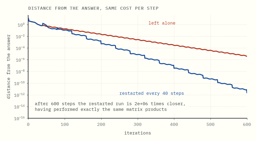
The iteration is unchanged, the two matrix products per step are unchanged, and so are the step sizes. Restarting every 40 iterations leaves it, after 600 iterations, about a million times closer to the answer.
Nothing was added to the inner loop. The averaging is vector work, invisible next to the matrix products. It is very close to a free improvement of six orders of magnitude, and it is why practical first-order LP solvers all restart.
(Real solvers choose the restart moment adaptively rather than on a fixed schedule, and there are stronger variants than plain averaging. The mechanism is the one above.)
Try it yourself → Sweep the restart period and find the best one, then check it against the 25.6 steps a revolution of the slow direction takes.
In one sentence. Averaging over a revolution cancels the rotation and keeps the drift, which costs nothing and is worth orders of magnitude.
11Does it get the right answer?
It should be checked against something that cannot be wrong.
The duality guide solved this workshop in exact rational arithmetic with a simplex method: 9 tables and 4 chairs, worth $350, with shadow prices of $6.25 a plank, $2.50 an hour and nothing for saw time.
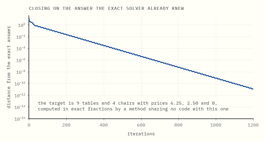
The first-order method finds the same plan, to fifteen significant figures.
It also finds the same prices, and that is more than a bonus. The prices are half of what the method is, so it produces the shadow prices without being asked. The duality guide's second problem is not something this method solves afterwards. It is the thing it was solving all along.
In one sentence. It converges to the same plan and the same shadow prices as the exact method, because the prices were half the algorithm.
12What it costs
Two costs, and they are the reason this has not replaced anything.
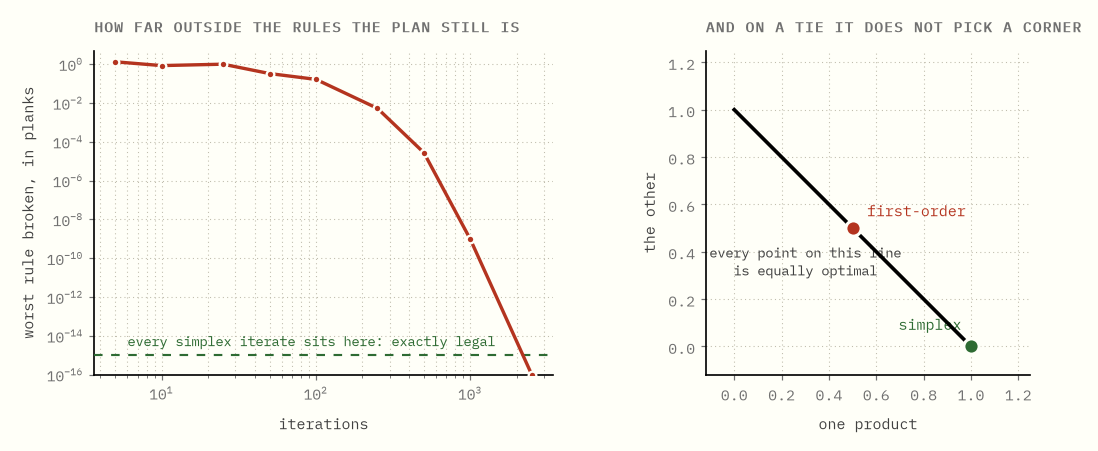
The plan is not legal until it has converged. A simplex iterate is always standing on a corner of the feasible region, so it is a plan you could actually carry out at every step. A first-order iterate approaches feasibility from outside. Ten iterations in, this one proposes a plan overrunning a shelf by 0.84 planks and claims to be worth $352.44, more than the true optimum, because it is cheating. It is worth more than any legal plan for the plain reason that it is not one: it is spending planks the workshop does not have.
The difference between that and a rounding error is a difference in kind. Stopping simplex early gives you a legal plan that might not be the best. Stopping this early gives you a number that is not an answer to your question at all.
And it does not return a corner. Take a problem where a whole edge is optimal, every point on it equally good. The exact method returns one of the two corners. The first-order method returns the middle.
Both are optimal, so for reporting a number it makes no difference. But branch and bound needs a corner: it needs a basis to warm-start the next node from, and a point in the middle of an edge does not give it one. Which is why first-order methods have transformed how very large linear programs get solved, and have so far changed integer programming much less.
In one sentence. You trade a legal answer at every step, and a corner at the end, for an inner loop that a wide machine can actually feed.
13Where this leaves things
The honest summary is narrower than the enthusiasm around it.
For linear programs large enough that forming and storing a factorisation is the binding constraint, a method whose entire inner loop is matrix-vector products is a different proposition altogether, and hardware built for bandwidth suits it. That is a real and important class of problem, and it was previously not solvable at all.
For everything else, the established methods remain established for good reasons: problems where a factorisation fits comfortably, problems needing high accuracy, problems that are really integer programs wanting a basis at every node. The chapters above are most of those reasons.
What has actually changed is that the answer to "which algorithm" now depends on the machine, in a way it did not for thirty years.
The specific benchmark numbers in this area move quickly, and none are quoted here, because a guide that dates in six months is worse than one that does not try. The primary sources, if you want the current state: the PDLP paper by Applegate and co-authors, the cuPDLP line of work, and Mittelmann's benchmark pages, which are updated continuously.
What the plain words are really called
| this guide says | everyone else says |
|---|---|
| operations per byte fetched | arithmetic intensity |
| the chart of what a machine can reach | a roofline model |
| a method made only of matrix products | a first-order method |
| the plan and the prices as two players | the saddle point / Lagrangian formulation |
| showing the prices where the plan is heading | extrapolation |
| the method of chapter 8 | PDHG, primal-dual hybrid gradient |
| the LP solver built on it | PDLP |
| average and start again | restarting |
| a plan that breaks a rule | primal infeasibility |
| a corner of the region | a basic solution |
Running the code
make bootstrap    # once, from the repository root
cd lp-on-gpu && make verify
There is no GPU in this repository and none is needed. Everything here is about the shape of the iteration, which is what determines whether a wide machine can be used at all, and that is visible at three variables as clearly as at three million. The tests check every claim above against the exact rational solver from the duality guide.